Matrices for a Financial Model

Scott Schaefer

Date: 2000 Feb 11

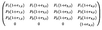
Rebalancing Matrix: $\begin{pmatrix} _{F_1(1+r_{1,t})} & _{F_1(1+r_{2,t})} & _{F_1(1+r_{3,t})} & _... ...t})} & _{F_3(1+r_{4,t})} \\ _{0} & _{0} & _{0} & _{(1+r_{4,t})} \end{pmatrix}$

Scott's Rebalancing Matrix: $\begin{pmatrix} _{F_1r_{1,t}+1} & _{F_1r_{2,t}} & _{F_1r_{3,t}} & _{F_1(1+r_{... ...}+1} & _{F_1(1+r_{4,t})} \\ _{0} & _{0} & _{0} & _{(1+r_{4,t})} \end{pmatrix}$

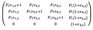
Growth Matrix: $\begin{pmatrix} _{1+r_{1,t}} & _{0} & _{0} & _{F_1(1+r_{4,t})} \\ _{0} & _{... ...,t}} & _{F_3(1+r_{4,t})} \\ _{0} & _{0} & _{0} & _{(1+r_{4,t})} \end{pmatrix}$

Allocation Matrix: $\begin{pmatrix} _{a_1} \\ _{a_2} \\ _{a_3} \\ _{w} \end{pmatrix}$

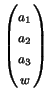
where F₁, F₂, F₃ are the percent allocation of the portfolio in each category ( F₁ + F₂ + F₃ = 1), a₁, a₂, a₃ are the actual amount in each category, w is the withdrawal amount at each unit of time, r_{1, t}, r_{2, t}, r_{3, t} are the percentage change of each of the respective categories at time t, and r_{4, t} is percentage change in inflation at time t.

In order to solve the homework, we can accumulate the rebalancing matrices for several years by simply multiplying them together and then multiply the allocation matrix this accumulated matrix. For example, we can determine the outcome over a five year period starting at 1926 by doing the following: [1930]*[1929]*[1928]*[1927]*[1926]*[A] where [A] is the allocation matrix.

It was conjectured in class that it was possible to do a one pass algorithm by accumulating these matrices and obtaining the next set of matrices by multiplying the left side by the next year and the right side by the inverse of the first year. Unfortunately, this is not the case because both reallocation matrices do not have an inverse. This is relatively easy to see because the determinant of the matrices is 0. Also, the first three rows are not composed of linearly independent vectors since they all lie within the same span.

It is clear from this model that the amount left in our portfolio after n years of withdrawing from it is linearly dependent on w, the amount withdrawn during each time interval. This is because the rebalancing matrices are accumulated independent of the actual amount withdrawn. Multiplying the allocation matrix by the final accumulated matrix yields a linear equal, dependent on w for the portfolio value. It is then possible to find the optimal w for that time interval by solving for w with the portfolio value equal to zero.

This model also allows for periods in which rebalancing does not occur. During these time periods, we simply multiply our accumulated matrix by the growth matrix instead of a rebalancing matrix. This allows us to rebalance our portfolio every two years or so instead of every year. This may be desirable because we must pay capital gains tax on the items that we sell.

A sensitivity analysis on the data that we obtain from this model was also proposed. If we assume that the data that we have for the percentage change in each category is off by a small amount, then we can write the rebalancing matrix as $\begin{pmatrix} _{F_1(1+r_{1,t}+\epsilon)} & _{F_1(1+r_{2,t}+\epsilon)} & _{F... ...4,t}+\epsilon)} \\ _{0} & _{0} & _{0} & _{(1+r_{4,t}+\epsilon)} \end{pmatrix}$

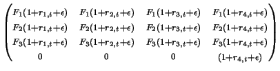
Actually, it is possible that a different $\epsilon$ be associated with each rate, but for simplicity's sake, we will consider them to be the same for the moment. The idea is that after we accumulate these matrices over time, this small error in our data can produce widely varying answers in our outcomes. This has not been proven yet though.