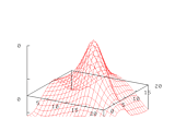
My research for the Masters Degree consisted of the extension of an algorithm for considering image segmentations in a probabilistic framework. The algorithm was developed by Steve LaValle for segmenting range images and was extended by Becky Castaño to considering grouping of symmetries in line drawings. I changed the method of integration from a numerical integration using Monte-Carlo methods to a summation over known samples, and implemented the algorithm in C++ to segment textured intensity images. My implementation uses a Markov Random Field model for texture. One thing this algorithm does is allows the segmentation algorithm to evaluate many possible segmentations of an image, and return the N most probable of these. A page from my thesis illustrates this concept. The abstract from my thesis follows.
Traditionally, the goal of image segmentation is to produce a single partition of an image. This partition is then compared to some ``ground truth'', or human approved partition, to evaluate the performance of the algorithm. This thesis utilizes a framework for considering a range of possible partitions of the image to compute a distribution of possible partitions of the image. This is an important distinction from the traditional model of segmentation, and has many implications in the integration of segmentation and recognition research. The probabilistic framework which enables us to return a confidence measure on each result also allows us to discard from consideration entire classes of results due to their low cumulative probability. Several experimental results are presented using Markov Random Fields as texture models to generate distributions of segments and segmentations on textured images. Both simple, homogeneous images and natural scenes are presented.
I believe that it is important for there to be more communication between vision modules than is possible in the typical segmentation goal, which is to return a single segmentation which is best in some sense. For example, if a satellite picture of crops is being looked at in the wrong spectral band, no information (or not much) will be available. The segmentation algorithm should note this and communicate this information to the higher level algorithm, which might try another spectral band or might run a test to see which band to look in. The idea is simply that often a single image isn't enough.
I've continued my work in uncertainty representation into the area of object tracking. My current work utilizes an optimal recursive data processing algorithm called the Extended Kalman Filter (EKF) to use information about the uncertainty in feature tracking and the uncertainty in the state estimate of an object to aid in tracking that object. For example, if I'm looking at the back of your head, I have much less confidence in my estimate of where you are looking than if I'm looking at your face. I have formalized this idea and implemented it into an object tracking system. Some example sequences are shown below.
The examples below look best on a 24-bit monitor. They seem (at best) a bit dim and grainy on an 8-bit (256 color) monitor. Sorry about that.
 |
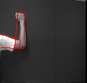
This sequence shows the tracking of an arm with 2 degrees of freedom active. The lengths of each link of the arm are initialized correctly, so the tracking progresses much as if the link lengths had been measured and set. In the estimation process, which is based on the same mathematically framework (extended Kalman Filtering) as the previous cases, the joint angles are modeled as moving with constant velocity and the link lengths are modeled as being unknown constants. The sequence above illustrates the initiation of tracking, but the full sequence is also available. |
 |
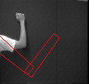
This sequence shows the tracking of an arm with 2 degrees of freedom active. The lengths of each link of the arm are initialized incorrectly, so the tracking progresses much as if the link lengths had been measured and set. In the estimation process, which is based on the same mathematically framework (extended Kalman Filtering) as the previous cases, the joint angles are modeled as moving with constant velocity and the link lengths are modeled as being unknown constants. The sequence above illustrates the initiation of tracking, but the full sequence is also available. |