Color Models
Color can add a lot of information to your plots. For this reason, the various plot styles of SwiftVis support a number of different mechanisms for determining the color of an element in a plot. While some of the plot styles have specific ways of doing this, many use a common set of models for calculating colors that are described here. Currently there are three different models for calculating colors that are part of the standard ColorModel class in SwiftVis. These include a gradient model, a solid color model, and an ARGB model.
Gradient Model
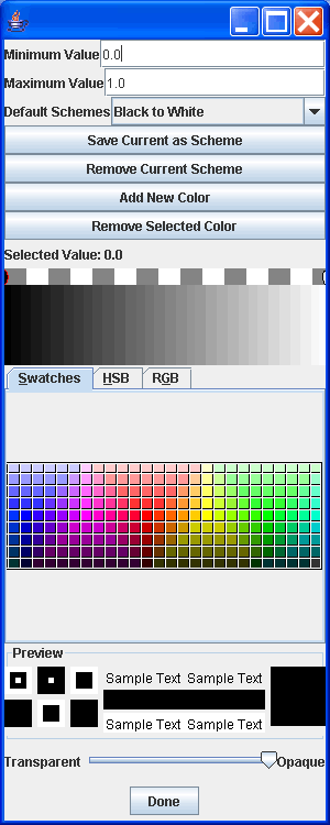
The gradient model is the default in most situations and the plot styles that don't support the full color model selection typically have some variation on the gradient model built into them. The full standard gradient model allows you to enter two formulas and set one gradient. The first formula gives a value that is mapped into the gradient to pick a color that might or might not include a transparency. The second formula can be used to have a transparency that has a different functional dependence. For that formula, a value of 1.0 or higher is opaque and 0.0 or less is completely transparent. The gradient settings are adjusted using a control panel like that shown below. This is the default settings for the gradient in most usages. The gradient allows you to set the minimum and maximum values that it is stretched between. Here they are shown to be 0.0 and 1.0. The drop box below that allows you to select from a number of pre-built gradients. You can add the current gradient to the saved list with the next button in the dialog box or remove a saved gradient with the button below that. The third and fourth buttons in the top section allow you to add and remove color points to the current gradient. Below that, the gradient is displayed with ovals marking where specific colors occur in the gradient.

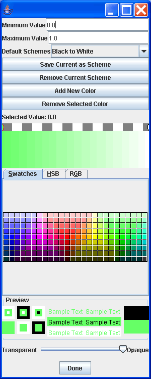
To help you understand how you can edit a gradient we will go through that process a bit and walk you through the steps. Note that the oval above the left end of the gradient is circled in red while the one at the right end is circled in black. The red oval indicates that it is selected. Whichever oval your mouse was closest to will be selected when the mouse enters that region of the dialog box. Clicking on the color selector will change the color. In the figure below we have changed the black to a pale green.

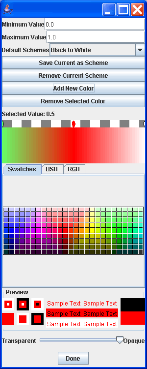
Now, while the first oval is selected, we click on the "Add New Color" button and a new oval is added between the two we have. By default it has a color of white. By moving the mouse near that oval we can select it and we then go down to change the color to red. That produces the dialog shown below.

Since the gradient is stretched from 0.0 to 1.0 and the new oval was placed in the middle, you can see it has a value of 0.5. You can click and drag the oval horizontally to change that setting. The slider at the bottom also allows you to make a given color in the gradient transparent. By default, all colors will be completely opaque. You can see when they are transparent because a checkered pattern will show through in the background of the region where the gradient is drawn.
By repeatedly adding and moving around colors you have the ability to create whatever gradients you want. If you create a complex gradient that you want to be able to reuse later on, simply use the "Save Current as Scheme" button. The new gradient will be at the bottom of the list during this and future executions of SwiftVis.
Solid Model
The second color model is the simplest. It simply lets you pick a single color. When you select this option from the drop box of a plot style that has complete color model options, you will get a single button that brings up a dialog box for selecting colors.
ARGB Model
The third model for calculating colors that is present in the full color model of SwiftVis is the ARGB model. This model allows you to specify four color formulas. These are evaluated to give red, green, blue, and alpha components for a color. A value of 0 will have that component completely turned off (that's transparent in the case of alpha) and a value of 1 will have it completely turned on (or completely opaque for alpha). This color model is probably most useful in a surface plot make with the rectangular surface plot style. In that usage, it allows you to easily overplot three distinct values by specifying them as the red, green, and blue values. It can also be used with the scatter plot style to allow you to color code points based on three distincts values. It isn't clear this is of the same value for scatter points, but if you find a plot that it works well for please let us know.