SwiftVis has capabilities for doing 3-D plotting. You do 3-D plotting using the same plot object that is done for 2-D plotting only you add in 3-D plot areas to the plot region. These function similarly to the 2-D plotting, but there are a few distinctions that are worth noting. The figure below shows a simple SwiftVis setup with a 3-D plot. The plot element of the graph is selected and in the properties we can see the properties of the Plot Area 3D object. There are five setting tabs in 3-D plots. This document goes through each in turn.
Data Sets
The first tab of settings for a 3-D plot, like that for 2-D plots, is the data sets tab. In this case the plot contains a test style as well as a scatter plot. The properties that are showing are for the scatter plot. The test style exist to allow you a quick test of 3-D plotting in SwiftVis to make sure that things are working. It contains three colored spheres and two triangles, as we will see below. A scatter plot, which draws spheres at specified positions, is also added in this example. The data coming in is a simple sequence of numbers with 100 values between -4*PI and 4*PI.
Currently there are only three plot styles for 3-D plots, but like 2-D plots, the code has been written so that more can easily be added. The plot styles that are useful for scientific purposes are the scatter plot and the surface plot. These are similar in nature to the scatter and surface plots in 2-D plotting. Note that the properties of the scatter plot allow you to specify formulas for the x, y, and z coordinates as well as sizes of the spheres. Color selection is made just as it is for 2-D plotting, though the alpha in the color is ignored in 3-D. Instead, 3-D plotting allows separate formulas for opacity and reflectivity. Different engines might handle these differently.
Engines
There are many ways to render 3-D graphics on a computer. The 3-D capabilities in SwiftVis were written in such a way to allow multiple different libraries to be used. The Render Engine tab allows you to select which engine you wish to use and change any settings associated with that engine. Currently SwiftVis supports two engines, both or which will work with any Java install and do all of their work on the CPU. There are plans to add other engines that will require other libraries to be installed, but which will use graphics card optimizations to do the rendering.
The two default engines are a CPU polygon engine and a ray tracing engine. By default the CPU polygon engine is used. This engine has been written in Java to transform objects from 3-D into 2-D so that they can be rendered with the Java2D library. The figure below shows our sample scene rendered with the CPU engine. Settings in the CPU engine allow you to alter how many polygons are used in the spheres and how wide a camera angle to use. This image uses the high polygon count and standard camera angle. This scene is lit by two light sources as will be discussed below. The time it takes to draw a scene scales with the number of polygons. For small scenes, this engine will refresh quite quickly. This scene has over 100 spheres, each made of 140 triangles and it renders in a fraction of a second on a 2GHz laptop. Using low polygon count spheres (diamonds with 8 triangles) this engine will render a fairly large number of data points quite efficiently.
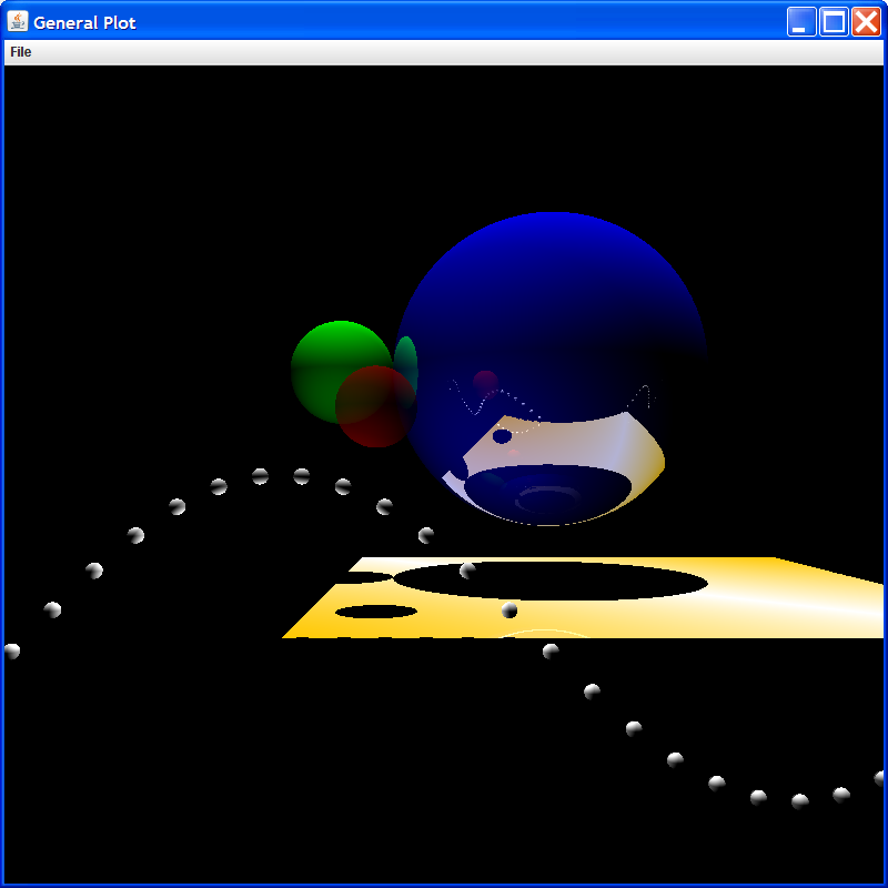
The second rendering engine that comes with a standard SwiftVis install is a ray tracer. The ray tracer will provide much higher quality output, but it is significantly slower. The time it takes the ray tracer to work scales with the size of the image and in odd ways with the number of polygons/spheres in the scene. For scenes with only a few elements, the ray tracer will be much slower than other engines. For scenes with many elements, the relative performance of the ray tracer improves though only because other engines will slow more than it does. Using the ray tracing engine, spheres are geometric spheres, not collections of triangles.
The figure below shows the same scene rendered with the ray tracer. While the CPU engine only draws polygons of the proper color and opacity, the ray tracing engine is able to include effects like shadows, reflection, and polygons that vary in color across their surface. The reason for having multiple engines is that you can set up a scene and get things looking the way you want using a fast engine, then switch to something that produces better output when you want to make a final figure.
The ray tracing engine includes a number of different options that impact the quality of the image that is produced. This figure was made with the default values. By default that ray tracer casts a single ray for each pixel. That can lead to aliasing, as seen in the image above. One of the engine options is to throw multiple rays per pixel. This can produce much more natural looking results, but note that render times will scale linearly with the number of rays cast. One can also set the maximum number of recursions for rays bouncing during reflection or scattered rays to pick up indirect lighting. Scattered rays add a lot of time to a rendering and probably shouldn't be used unless you really want that effect. Like the polygon engine, the view size can be set to alter whether the camera wider of narrower field of view. It is worth noting that the ray tracer is parallelized so if yo uhave a machine with multiple cores, adjusting the number of threads that SwifVis uses in the Options menu can significantly improve the rendering speed.
To see a more practical example of what you can do, see this animation of a ring patch simulation. Auto processing was used to quickly process the frames which were joined together using convert (command line ImageMagick tool).
Lights
The lights tab allows you to set/adjust three types of lighting in the scene. The first is ambient lighting, which illuminates everything evenly. The second is point source lights. These are like light bulbs that can be moved through the scene. By default, new point lights are placed at the origin with a color of pure white. You can click on a light and select edit to change it's location and color. The location can be specified with formulas that will be evaluated on the first element of the input. This will allow you to move a light source around in animations. As with a light bulb, the further you are from it, the less light from it hits a given object. For scenes of different scales, this effect can be adjusted properly by editing the light length scame in some engines.
The third light setting is a directional light. This works like having a bright point source at infinite distance so the light rays come in parallel. Location does not alter the intensity of this light on an object, only the orientation of the surface to the direction of the light. When you create a directional light, by default it is pure white and oriented in the negative Z direction. You can click on the light and click edit to change the direction and the color. As with the point light, the direction can be specified with formulas so that the light orientation moves in an animation.
The scenes shown above were illuminated with one point light and one directional light, both with the default settings.
Camera
The fourth tab is the camera tab. In a 2-D plot you specify what should be shown in the plot by adjusting the axes. In 3-D you alter the location and orientation of a camera that looks over the scene. In the SwiftVis 3-D plots this is controlled with the settings in the Camera tab shown in the figure below. There are three vectors that specify the camera location and orientation. The location of the camera is specified by the center values. The forward values specify the direction that the camera is looking from that given location. The up values specify another vector that is up in the image. Forward and up should generally be perpendicular to one another. Having them set otherwise will lead to interesting visual effects in some of the engines.
The entries for center, forward, and up can all be made as general formulas. These are evaluated on data element zero of the inputs. This allows the camera to move around through the scene in an animation.
Of course, specifying the view of a 3-D scene by typing in the placement and orientation can be rather tedious. One of the advantages of 3-D representations of data is being able to look at it from different angles. For this reason you can move the camera around using arrow keys and the mouse. The setting allow you to adjust some of the parameters for how this movement happens. A good way to work with a 3-D view of your data is to start with a camera position that overlooks your data set then manuver the camera to where you want it ot be with the kayboard and mouse. The location of the camera can be moved using the arrow keys along with Page Up and Page Down. The Move Step Size setting determines how far the camera will move on one press of a key.
You can adjust the orientation of the camera using the A, D, S, W, Q, and E keys. The A and D keys turn to the left and the right. The S and W keys rotate the view up and down. The Q and E keys roll the camera to the left and right. Combining these with the movement keys allows you to place the camera anywhere in 3-space with any orientation. The Key Rotate Step Size determines how far the camera will rotate, in radians, on a single key stroke.
Of course, sometimes it is helpful to rotate the data. SwiftVis will give you the illusion that you are doing this by pivoting the camera around as the click and drag the mouse. The last two settings deal with this capability. The point of rotation is taken to be a point a specified distance in front of the camera. The Mouse Rotate Center Distance setting allows you to adjust how far in front of the camera the rotation point should be. You can also turn off the redrawing on a drag. When this is off, the scene will only be rerendered when you have released the mouse.
For the keys to work the drawing will have to have focus. This can be achieved by clicking on it. Remember that some engines take a long time to render the image. For navigating around the scene you probably want to use the fastest engine you can. Also, it should be noted that moving the camera with the keys or the mouse will replace any complex formulas used in specifying the camera location or orientation with simple numeric values.
Geometry
This one setting is just like that for 2-D plots. You get to specify what fraction of the plot region is covered by this particular element. This allows you to place 2-D and 3-D plots side-by-side in the same window.