Finding Particles in Resonance
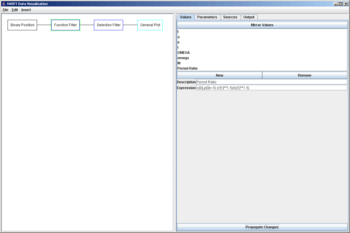
The objective of this tutorial is to find all of the particles that are in N:1 inner mean motion resonances with Juptier in a particular bin.dat file and produce a plot that shows that information in a manner that is at least somewhat meaningful. To being this tutorial we add a Binary Position elements to our graph, select it, and read in the file that we are interesting in. Then we need to add a Function Filter to the graph as well using Insert Filter or Ctrl-F. After selecting the Function Filter click the "Mirror Values" button, then click on the "Parameters" tab and click on the "Mirror Parameters" button. This will set it up so that all the values of the bin.dat file are passed through. Now go back to the "Values" tab and click the "New" button to add a new value. We will call this value "Period Ratio" and the formula for it is "{v[0],p[0]=-5} (v'[1]**1.5)/(v[1]**1.5)". This is a rather complex formula so we should discuss what it does. The curly braces at the beginning indicate that we are using a group and selecting special elements of this group. The grouping is defined by elements that have the same value of v[0] (the time in a bin.dat file) and out special element is the one with the first parameter equal to -5 (that happens to be Jupiter in this simulation). The rest of the formula is just the semimajor axis of Jupiter (v[1] is semimajor axis in the bin.dat file and v' indicates a value from our special element in the group) raised to the 1.5 divided by the semimajor axis of the test particle raised to the 1.5. The figure below shows that formula entered into the function filter.

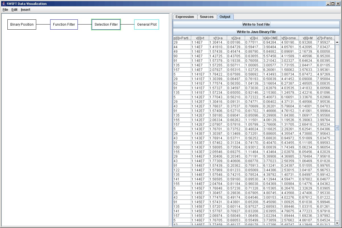
We can click on "Propogate Changes" and look at the Output tab to see the new elements that this will put out with the ratios of the periods. We now want to select only those test particles for which this ratio is close to an integer value. We do this by adding a Selection Filter and using the following formula: "abs(v[7]-round(v[7]))<0.05 and p[0]>0". The first part says that the ration must be close to an integer value (within 0.05 in either direction) and the second part says that it has to be a test particle just so that Jupiter itself doesn't come through in the data. Again, looking at the Output tab after clicking on "Propogate Changes" allows us to see the effect of this. The figure below shows the output from the Selection Filter using our example data file.

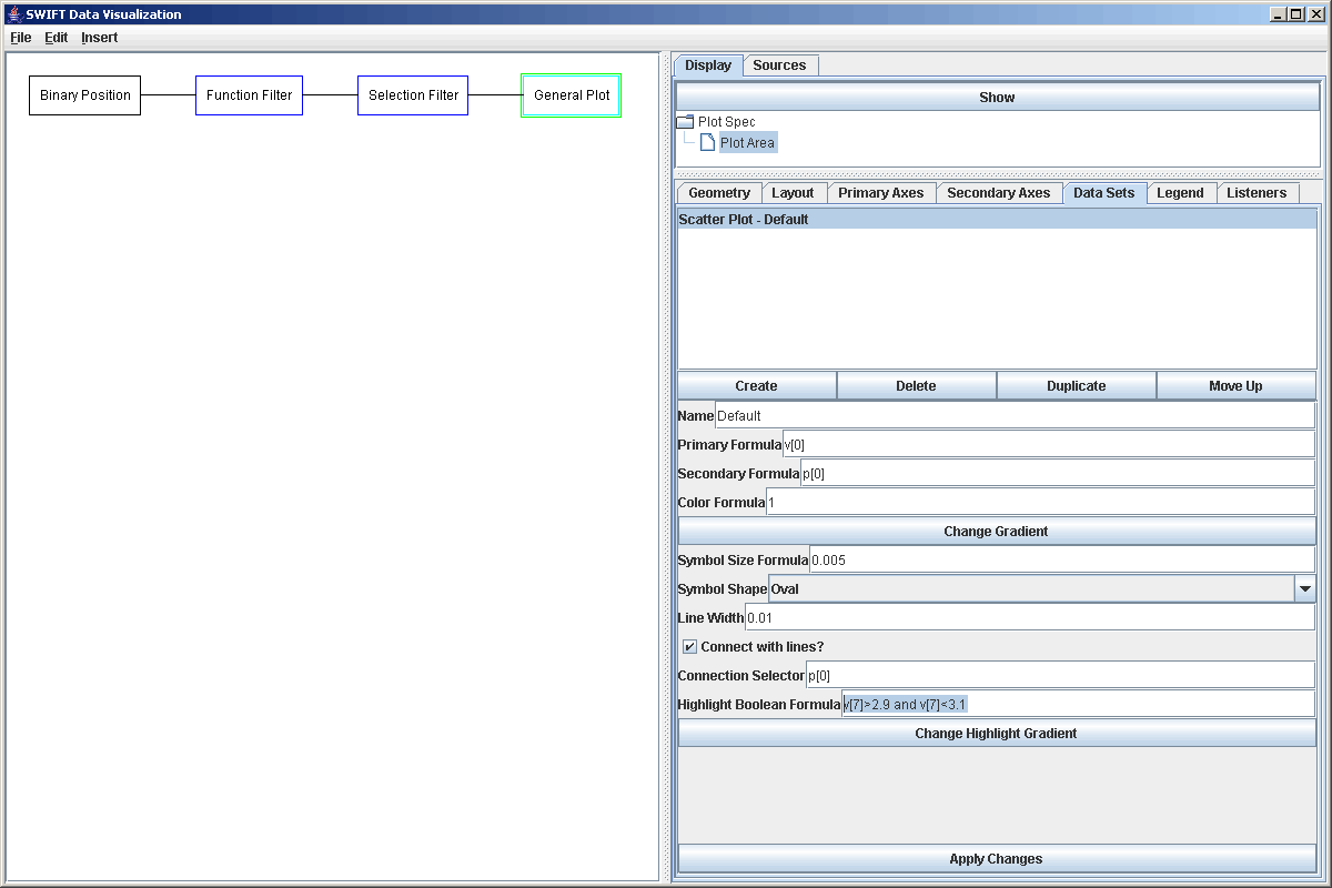
Lastly, we want to plot this up in a way that easily lets us see when particles were in resonance and for how long. We add a Plot to the graph and add a Plot Area into it. Going to the Data Sets tab, the Scatter Plot style is fine to use, but we need to edit the formulas some. For the secondary formula, we will use p[0], the number of the test particle. This way the plot will have one row for each particle. To help make the rows more apparent, we select "Connect with lines?" and set the "Connection Selector" to p[0]. This way, there will be lines drawn between all of the data points for the same particle. Just for fun, we can also highlight all of the particles that are near a certain resonance. To do this we edit the highlight formula to be "v[7]>2.9 and v[7]<3.1", so we are highlighting things in the 3:1 resonance. Then we change the highlighting gradient and make the upper end color red so that those point will stand out. The figure below shows the properties of the Scatter Plot after we have made our changes.

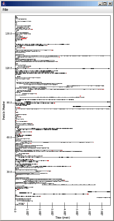
Now we add some labels to the axes to help make thing more understandable, and we get the following plot. Every timestep when a particle was near a resonance with Jupiter is denoted by a dot. The lines show the time period from the first time a particles was in resonance to the last time it was in resonance.

As an alternate approach to seeing that particles are in what resonances, you can use v[7] as the color formula and set the gradient to go from the minimum N to the maximum N that is expected with at gradient the is either a spectrum or something from black to another color.