A Global Simulation of Saturn's F Ring with Prometheus and Pandora

These animations show different views of a global simulation of a system similar to Saturn's F ring. The simulations include interparticle collisions, but not particle self-gravity. There are two perturbing moons that have separations from the rings, eccentricities, and masses similar to Prometheus and Pandora, but the exact orbits are not derived from observations. The ring material begins the simulation as a circular ring with Gaussian radial distribution 14 km across.

The animations show 20 orbits each with 10 frames per orbit and 0 being the beginning of the simulation. The Prometheus-like moon is interior to the ring and moves to the right relative to the ring material while the Pandora-like moon moves to the left significantly faster. In addition to showing the optical depth for the entire simulation, the animations show several other views of the data. There are small regions at from from -1.4 to -1.6 radians and from 1.4 to 1.6 radians. For these regions the optical depth is shown along with the guiding center optical depth and the eccentricity binned in guiding center space. There are also radial profiles taken at roughly -PI/2 and PI/2. Note that for the surface plots, the units on the axes represent the exact same lengths so the aspect ratio, even on the plots showing smaller regions, are far from 1:1.

The animations are in animated GIF format for maximum compatibility, but this makes them fairly large which is why they are broken into difference pieces. More pieces will be added as the simulation progresses.

Orbits	AVI	GIF
0-19	16 MB	26 MB
20-39	16 MB	32 MB
40-59	17 MB	38 MB
60-79	17 MB	39 MB
80-99	18 MB	41 MB
100-119	17 MB	43 MB
120-139	18 MB	42 MB
140-159	18 MB	41 MB
160-179	17 MB	40 MB
180-199	18 MB	41 MB
200-219	18 MB	40 MB
220-239	18 MB	37 MB
240-259	18 MB	37 MB
260-279	17 MB
0-279	200 MB

The following animation is from another simulation with slightly different initial conditions set up to produce a perturbation in the ring similar to what occurs in the real system. Only a single mplayer AVI file is given for this simulation. Movie File

The exact details of these types of simulations are sensitively dependent on the simulation setup, particularly values like the synodic period. The integer m number of the nearest resonance is much less significant than where the ring is between resonances. That is because the fractional part of the m number determines what ring material will get the largest perturbation from the moon relative to the material that got that perturbation in the previous kick.

Eccentric Ring

More recently we have worked on trying to incorporate the last pieces of realism into the simulation and match as mcuh of the physics as we can. This includes making the ring eccentric and making the moons inclined. It also includes adding particle self-gravity and making the distribution of particles wider. In the simulations above, all the particles collapse down into a single core. From earlier work we can say that this is because the width of the initial distribution, measured in orbital radii, is not significantly larger than the forced eccentricity. This new simulation uses a much broader distribution. Instead of having particles cover 10-20 km radially, this simulation has particles spread across 140 km radially. It is a Gaussian disribution so that the central density is much higher than on the wings, but with this distribution, we expect to find that the core is not able to pull in all the particles.

There is another fundamental change in this simulation. With the inclusion of self-gravity, this simulation also turns the moons into "normal" particles. Granted, they are very big, but they experience full gravity and collisions like any other particles. So if Prometheus were to come in close enough to skim material from the edge of the ring distribution, the simulation would not have a problem doing that. This type of work was enabled by code alterations I made to do granular flow work with Josh Colwell. I refer to the method as the lock graph which gives a more dynamic approach to locking collisions during the collision handling phase of the simulation.

Of course, there has to be a drawback to making this so realistic. Indeed there is and it is computation time. Early in the simulation we are seeing about 7 hours of run time per orbit using 96 cores. That isn't horrible, but the simulation will need to run several hundred orbits to get past the transient phase. The figure below is one time step from the simulation, just 4.5 orbital periods in. All units are lengths in R_0, the semimajor axis of the ring. For the global plots, the eccentricity surface has been plotted with a downward offset.

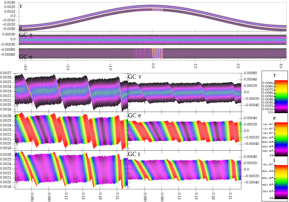
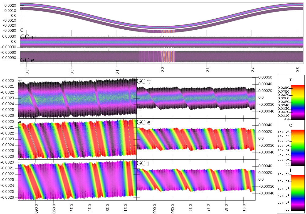
What will be interesting to see is how much negative diffusion occurs and what range of semimajor axes it pulls in material from to the core. The complement of that set will be the material left out in the apron. It will also be interesting to see if negative diffusion will create strands of material out there or if the optical depth will be too low. The image above shows the ring near closest approach to Prometheus when the Prometheus wakes are experiencing compression. Here is a second plot showing them half an orbit later in rarefaction.

It is probably worth a few sentences to describe how these plots are made. These are plots of what I refer to as particle binned data. Full simulation dumps for this simulation are 2.8GB each. That makes them rather difficult to work with and it is hard to store many of them for analysis because they take up too much disk space. To get around this, I more frequently write out binned data sets. A normal binned data set will make a grid and calculate average values in that grid. This has some drawbacks and is especially ineffective for a simulation where the ring is eccentric. The particle binned method bins particles azimuthally in the normal way, but then sorts the particles by the radial value in those bins. It then outputs averages for particles in groups from the sorted set. This has the advantage that it only covers the radial region needed and is higher resolution in areas where there are more particles. Because it is binned, the files are significantly smaller than full dumps making them easier to store and work with. We can still go back to the full dumps when we want to look in detail at specific regions, but these files make it a lot easier to find those regions. One other point to specify is that the e values aren't simply e. They are abs(e-0.00233). The constant in there is the initial eccentricity given to the whole ring. This has to be subtracted out so we only see the effect of the perturbation.

I now have a bunch of frames doing the surface plots shown above as well as another type of plot showing particle streamlines. You can look at all the different frames here. I also have movies of the surface plot and the streamline plot. One problem with the eccentric ring is that the axis range keeps changing which makes the movies less smooth. The numbers on the images are the step count. There are 200 steps per orbit so you can easily figure out how far into the simulation each frame is.

The streamline plot is intended to look at negative diffusion in the ring. This is a process that occurs when streamlines intersect and slightly overlap. Because of the low optical depth of this simulation, they experience a fair bit of overlap. The left panel in the plots shows the streamlines, colored by their optical depth. The right panel shows locations of guiding center bins as partially transparent dots. The transparency allows you to see when they are stacked on top of one another. The process of negative diffusion is a migration of the semimajor axes of particles toward areas of higher optical depth that happens abruptly when the streamlines cross. We believe this process is what holds the core of the F ring together. It is likely also responsible for maintaining the narrow rings around Uranus and Neptune as all it needs in ring material and a significant perturbation.