Using Discard Information
Perhaps the second most used data file in the SWIFT package behind the bin.dat file is the discard file. This file records when test particles are removed from the system due to either a close encounter with one of the massive bodies or because it went to close to or too far from the Sun. The primary use of this data file is for finding which particles were discarded in different ways. In this tutorial we will set up a SWIFTVis graph that pulls information from both a discard file and a bin.dat file. We will look at the discard file itself, then use the information in the discard file to select specific elements in the bin.dat file for further analysis.
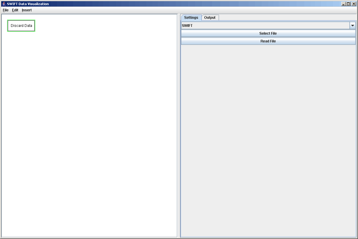
The formats of the discard files for SWIFT and SWIFTER are a bit different. Due to the fact the SWIFTER is not yet in widespread use, we will be dealing with the SWIFT format here. SWIFTVis does not pull in all of the values stored in a SWIFT discard file, only the most generally used ones. If you want other values, you could use the general data source to read in the discard file will all the values that you want. The main values that are left out are the istat and rstat values for indexes above 3. This leaves most of what people are actually interested in. To begin this tutorial, we add in a Discard File by going to Insert > Data Source or pressing Ctrl-D, then selecting the Discard File option. Clicking on the Discard File element in the graph we see the few options that are available for it. You can specify if you will be reading a SWIFT or SWIFTER data file, pick what file to read, and actually do the read. The figure below shows this.
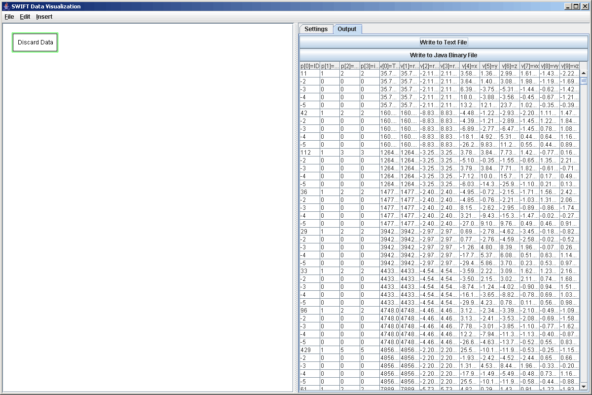
After selecting a file and clicking to read it, we can click on the Output tab to make sure that we got the information that we wanted. This not only shows us that the file was read in properly, but the column headers can help us to remember which values and parameters are what. A view of this for our discard file is shown in the figure below.
Now that we have a discard file, we want to do something with it. There really isn't much that we can plot with a discard file alone that makes sense. We can pass it through a filter or two to quickly see some information. For example, we could pass this through a selection filter to see only the test particles that were discarded because they came to close to a particular planet. To do this we create a selection filter and enter the formula p[2]=3. In this simulation, massive body 3 is Saturn so we can quickly see how many particles were discarded due to a close encounter with Saturn. Remember to click "Propogate Changes" or the output panel will be blank. The figure below shows that filter added and the output results when we do that selection.
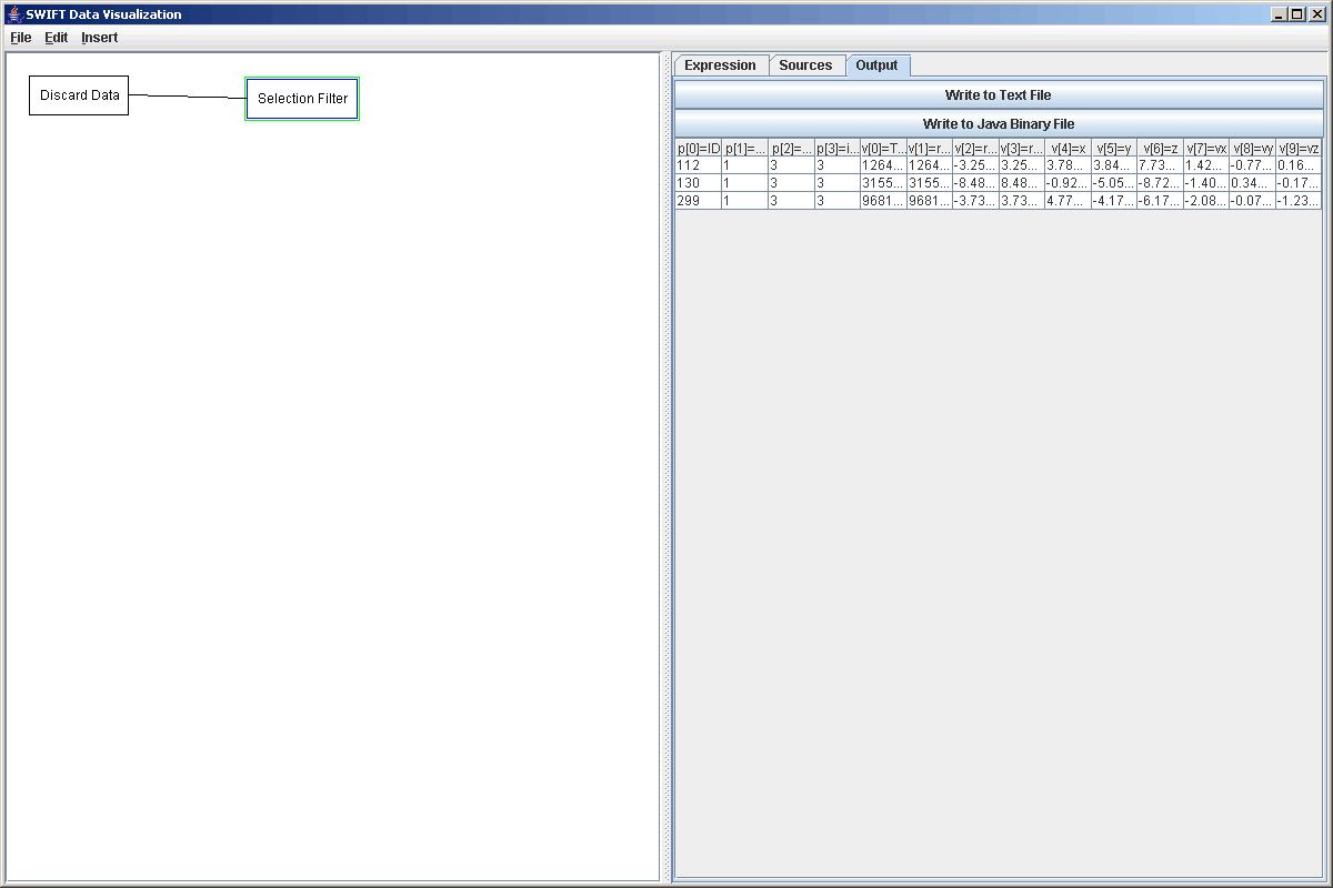
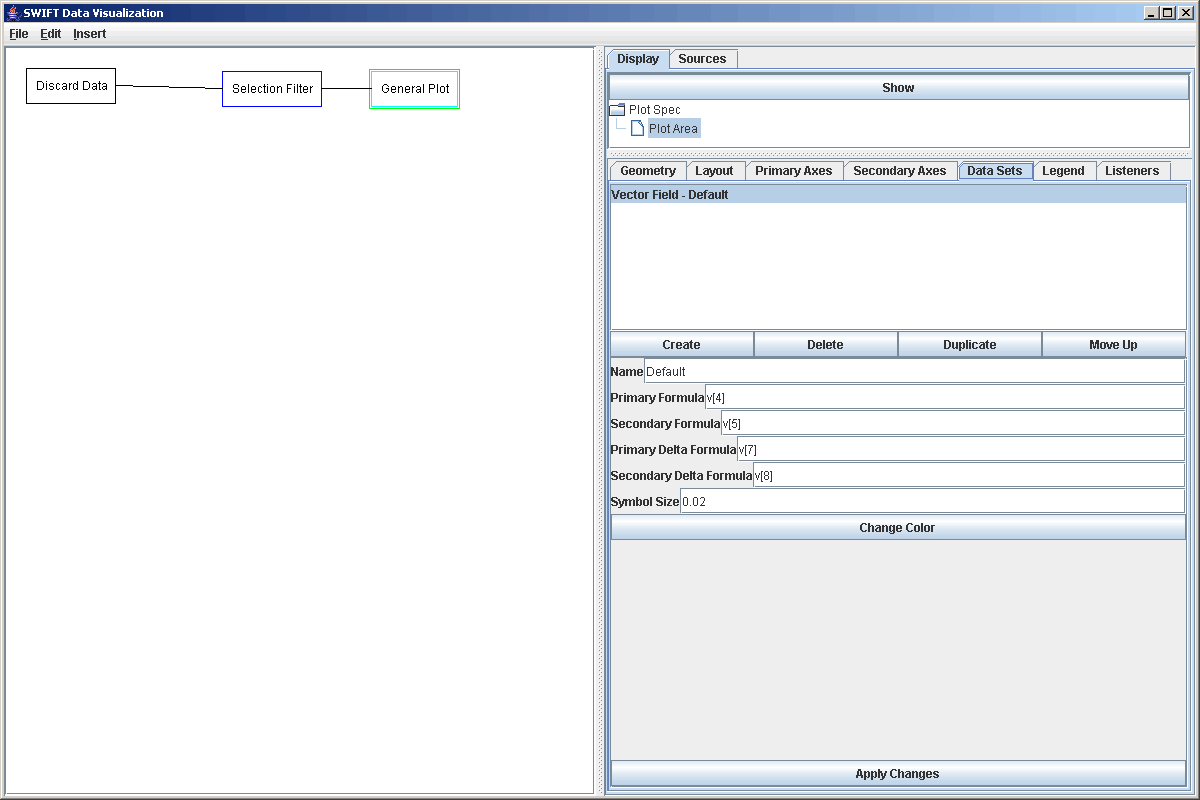
As you can clearly see in the figure, only 3 particles were discarded because of close encouters with Saturn. We can quickly change the selection expression to p[2]=2 and see what test particles were discarded because of close encounters with Jupiter. In the discard file that we used, there were 11 such test particles. Though it likely won't show that much, we could quickly put this into a plot to demonstrate a different bit of plotting functionality. We create a plot and click Add Plot. Then select the Plot Area and go to Data Sets. We want to create a vector field and delete the scatter plot. Now in the vector field properties change the primary and secondary formulas to v[4] and v[5] as those are the x and y coordinates, and change the primary and secondary delta formulas to v[7] and v[8]. These changes are shown in the figure below.
For visual clarity we also changed the symbol size to 0.02. This produces the plot shown below. (We also played with the ranges on the axes to get a square that completely encloses the points and vectors.) Though it might not having any meaning, this plot does clearly show us that at the time of the discard, all of the particles in this simulation that encountered Jupiter were heading outward in their orbits or were moving mostly azimuthally. Of course, if we wanted to see the same plot for Saturn, we need only go back and change our formula in the selection filter and propogate the changes. The plot will automatically update.
Of course, people are typically interested in using the discard file to select elements from another file, such as the bin.dat file. To do this, we need to use a different type of filter. The selection filter can have multiple inputs to it, but doesn't do what we want here. For it to have meaning the two input files must be "parallel" in that the ith element in one needs to relate to the ith element in the other. That is certainly not the case for a discard file and a bin.dat file. To produce the results we want here, we need to use a Key Selection filter. Before we can use that filter though, we need to load in a bin.dat file. The bin.dat file for the simulation in question was 1GB in size. SWIFTVis does a number of things that can help you in dealing with files this large if your machine does not have enough memory to load all of it at one time. In this case, the machine used to write these tutorials only had 512MB of RAM so storing the entire file is not feasible. If you truly want to be pulling data from the entire file, the Binary Position source that reads the bin.dat file does cacheing automatically for you. How much it caches at one time depends on a setting in the options. It is only ar ough value, but you should make it small enough that it won't push your machine to the point of swapping. If you depend on this, however, you should expect slow performance, because anytime you read something outside of the buffer, you must make a significant read from disk first. In this situation, the first thing you want to do is pass the data to a filter that you set to cut down the data to a much smaller level. The filters don't cache so if you use a filter like a Function filter that doesn't cut out anything, or use a selection filter but don't cut out much, you can expect SWIFTVis to die running out of memory. On the plus side, after you have editing the filter and propogated changes, any other analysis or plotting you do pulls from the filter and wont go all the way back to the source to hit disk.
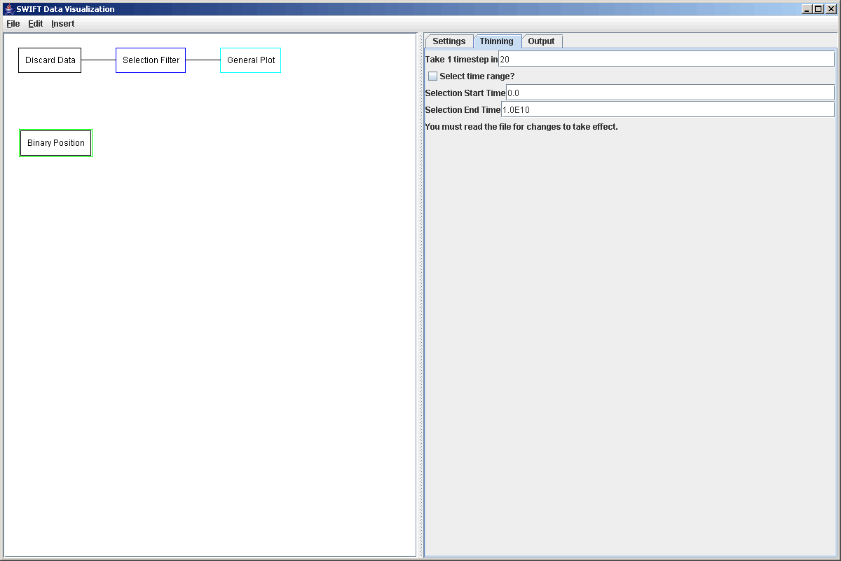
In this case, we actually don't need quite all of the data from the bin.dat file, so we use some options in the Binary Position buffer to automatically thin things out for us. The Binary Position source has a tab labeled "Thinning". The options here basically let you do the same thing that a Thinning Filter would do or a limited selection filter that only selects a certain time range. The thinning drops out all but 1 in a specified number of timesteps. That is what we will use in this example because while we want to see the entire timerange, we don't really need to full detail in the data. This simulation goes for 4e9 years. If later we decide that we want to see the full details on some smaller chunk of time we can simply edit the thinning parameters and reread the file. To see full details for a single particle or a small group of particles, we could set the thinning to read in everything and then pass it through a Selection Filter that takes only the particles that we are interested in. The screenshot below shows the thinning parameters that we are using for this example.
Now that we have read in the bin.dat file and we have our discard source, it is time to add in the Key Selection Filter. You can add this with no elements selected from the graph, with the discard source selected, or with the binary source selected. You will have to at least one new connection and the order you add them matters in how the formulas are entered. We connected to the discard source first and the binary source second. The reason being that we have to enter two formulas that relate to the discard source and it means a bit less typing. If you can't remember what order they were entered in, just go look at the Source tab and you can see them in order. The first formula we have to enter in the Key Selection Filter is a boolean formula that tells what elements to select to get keys for. In this case, we want to select all the test particles that were discarded because they ran into Jupiter so we enter p[2]=2. Remember that by default values and parameters are pulled from the first data source so that is shorthand for d[0].p[2]=2. The second formula we have to enter is a data formula for the value of the key that we want to use. The idea is that the key values will match between the two data sets. In this case, the key we want is the particle number, or p[2]. The last settings tell the Key Selection Filter which source to pull elements from, and what formula to use for calculating keys on that data source. The figure below shows the properties for the Key Selection Filter that were used here.
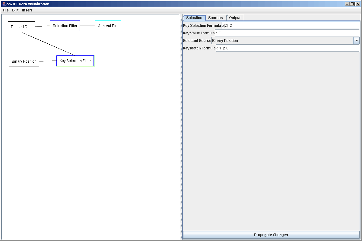
Notice that the last formula explicitly gives the data source being pulled from as d[1], the second source. We can click on Propogate Changes and then look at the output panel to see if it worked. The figure below shows the view of the output panel. Comparing this to the output of the selection filter we made earlier, we find that we do indeed have all of the particles that were discarded by Jupiter and we have their full histories as read in by the Binary Position source.
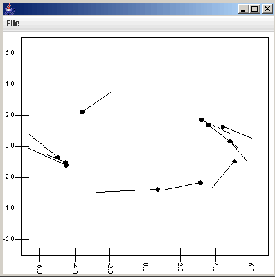
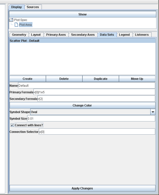
Now, just to do something with this data, we can send it to a plot and look at the scatter plot of the eccentricities of those particles over time as well as the eccentricity vs.semimajor axis. To do this we simply do Insert > Plot, select the plot, and click add Plot. We get the scatter plot by default, but we need to edit what it is plotting and add a second scatter plot. For the first plot, we want to plot v[0] as the primary, but to get values that don't have 6 digits in them we plot v[0]/1e5. For the secondary formula we use v[2], the eccentricity. If you show the plot and click Apply Changes at this point you get something that is rather hard to interpret because of the numerous particles. To help sorce this out we can use another option of the scatter plot. The last two options are a check box for drawing lines and a formula for specifying what should be connected. We want to select the drawing of lines, and use the formula p[0]. This will put lines between data points of the same particles. The following figures show the properties panel and the plot for that. (Note that since this tutorial was made, more options have been added to the scatter plot.)
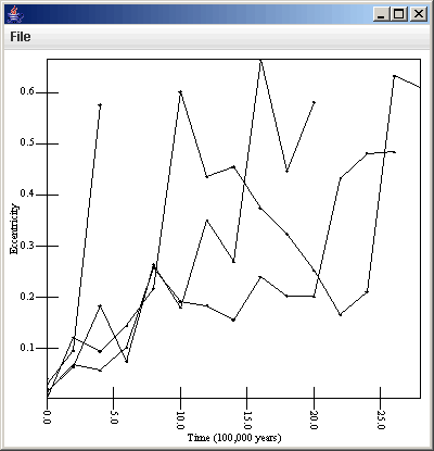
To make things look a bit nicer labels were placed on the axes. This isn't required for fast analysis, but helps people understand what they are looking at.
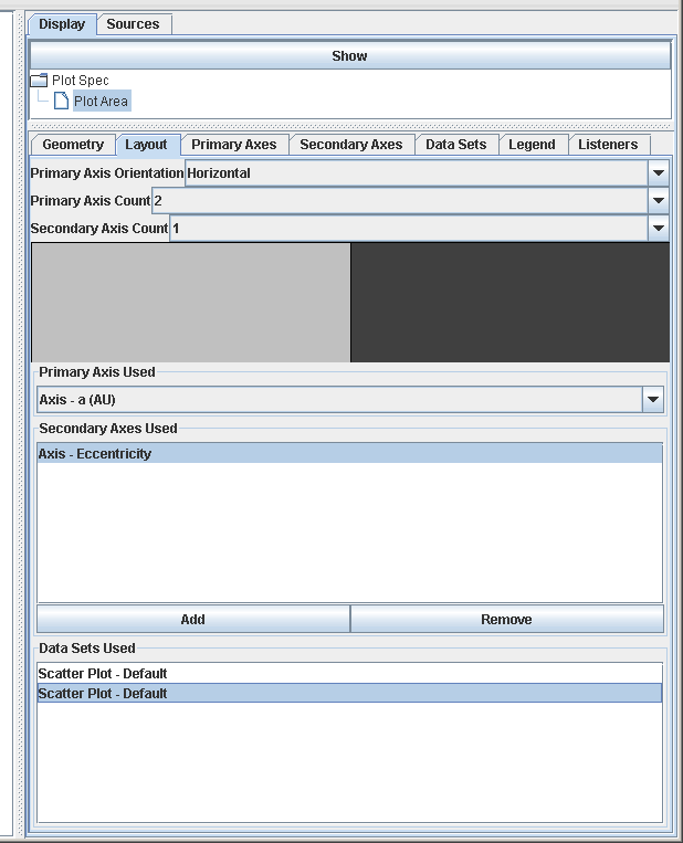
Now we simply need to create a second scatter plot and have it plot v[1] for the primary axis and v[0] for the secondary axis. Lines might be helpful here as well. So that we don't share an axis or overplot, we will create a second primary axis with the lable "a (AU)" and under layout set the primary axis count to 2. We can click on the right panel of the gray plot and change what primary axis is used with the drop down box. Lastly, we click on the second scatter plot at the bottom of the properties panel and our plot updates. The figures below show the layout in the plot properties panel, and the plot that is generated.
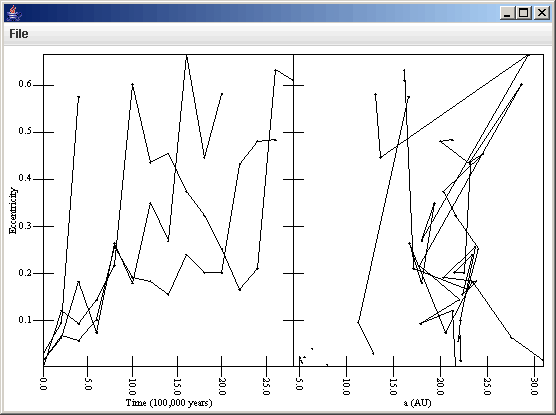
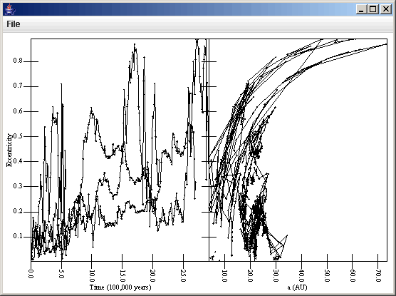
The plot now looks decent and shows the information that we want, but the data is rather sparse so the lines jump around a lot and we can clearly see that for the bodies we are interested, none survived close to the 4e9 years of the integration. So we can go back and change the Binary Position source thinning parameters and keep 1 in 1 timesteps, but turn on the range selection and set the maximum on the range to 3e6, which includes the time range of our particles that encountered Jupiter. After making this change we go to the Settings tab and click "Read File" and the plot automatically updates to the figure shown below which has the full time resolution of our bin.dat file for this simulation.
This tutorial have shown you how to include the discard file output in your analysis using SWIFTVis. The Key Selection Filter plays a significant role in this by allowing you to make selections on one data source based upon values in another data source. We now turn our attention to some aspects of SWIFTVis that don't directly relate to SWIFT. This begins by looking at the General Data Source, which allows you to read information from a wide variety of text and binary input files.
For more information on the topics presented in this tutorial, you should look at the full descriptions of Discard File Source, Key Selection Filter, Selection Filter, Plot, and Scatter Plot.