Reading Data from General Sources
While SWIFTVis was obviously written to help with the analysis of SWIFT data plots, it has the power to be a general data analysis and visualization tool and can also be used with other sources of data. In this tutorial we look at a Source in the SWIFTVis package that can be used to pull in more random data files in text or binary formats. Sources of this type can be put into a SWIFTVis graph just like any of the sources that are specific to SWIFT and be passed through filters for plotting. To demonstrate this, we will show how SWIFTVis can be used to look at data from three different data files that are output by a different simulation code that has been used to do work on planetary rings.
The source that we are introducing here is the "General Data" source. This source is intended to work with most space delimited or binary data files. To begin with, we want to add an element of this type into our graph. We go to Insert > Data Source or Ctrl-D and select the "General Data" option from the dialog box. Selecting this element we get a properties panel that allows us to enter the speficiations for reading the file, select a file, and actually read from the file. The figure below shows this property panel. The top option is between simple text format and special format. If you select simple text, there are no other options. This format simply reads each line of the file as one element. If the number it reads is an int, it becomes a parameter. If it is a floating point value it becomes a value. Anything other than a number will cause an error.
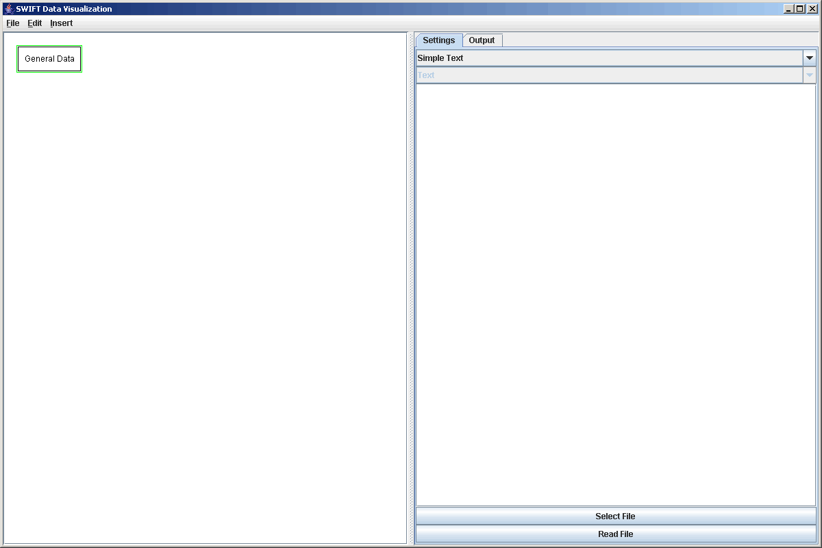
I special format is selected, then the second drop box and the large text area are enabled. The drop box allows you to specify whether the file you are reading from is a text or binary file. The text area allows you to enter a format string. The format string tells SWIFTVis the details of how the file should be read. For a full discussion of these options, go to the General Data page. Here we will only introduce the aspects that are needed to cover the examples we are interested in. All three of the files that we will read will use the special format.
The first file we want to read stores binned values for a parameter as the simulation cell moves downstream. The format of the file is an azimuthal position (Y) followed by 100 numbers for the value of that particular value for all the particles that were in a given bin. If the value is the optical depth, then each value gives the combined cross sectional surface area of the particles in the bin divided by the area of the bin. If the value is eccentricity, then the values will be the average of the eccentricites of all the particles in that bin. The file is stored as a text file and we could inevitably read it in using the simple text option. The main problem with this is that it would give us 101 values in each element that would be very hard to pull apart. Just like time values are shared between all elements from the same timestep in a bin.dat file, here the 100 values basically share the same Y value. In SWIFTVis this means that we want to have elements with 2 values in them. v[0] is the Y value and v[1] is whatever was binned in the cells.
The format string to read in this data file is "v[0]=r {100 v[1]=r}". Let's look at this. There are two main constructs that you see. The v[0]=r and v[1]=r tell the general data source to read in a floating point number (r for real) and store it into the specified value. If we were reading an int we could use "i" instead of "r". To store a parameter we use p[#] instead of v[#]. The other construct is the curly braces. These produce a subgroup that is read multiple times. In this case, we are reading v[1] 100 times. Every time we hit the end of a close curly brace in a format string, an element is added to the source. So the way this format string is read is, read a real into v[0], then do the following 100 times, read a real into v[1] and add an element. The whole process is repeated until we get to the end of the file.
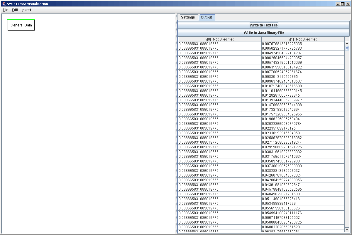
After entering the format string we select the file and read the file. By clicking on the Output tab we can see that it worked. This is shown in the figure below. If you were able to scroll down, you would find that there are groups of 100 elements that have the same v[0] with different v[1]s.
It is worth taking a bit of time just to do something with this data as it gives a good excuse to introduce another of the filters in SWIFTVis. One of the significant drawbacks of this data format is that while all of the v[1] values in a group are taken for bins at different radial positions, there is nothing in the data file that makes this clear, much less tells us what values those are. We need that information to make a surface plot of the data, which is our goal here. The bins happen to be evenly spaced so we can make a big step in the right direction if we can enumerate the elements of the groups. We can do this in SWIFTVis with the Group Numbering Filter, which was created for this specific data format, but can be used to enumerate the elements of any datafile where elements are grouped and will enumerate the groups themselves. To use this we simply add a Group Numbering Filter with Insert > Filter or Ctrl-F. By default, it makes the groups based on consecutive equal values of v[0]. That happens to work well for what we just read in and would work equally well for a bin.dat file where v[0] is the time value of an element. That formula is the only thing that can be specified for this particular filter.
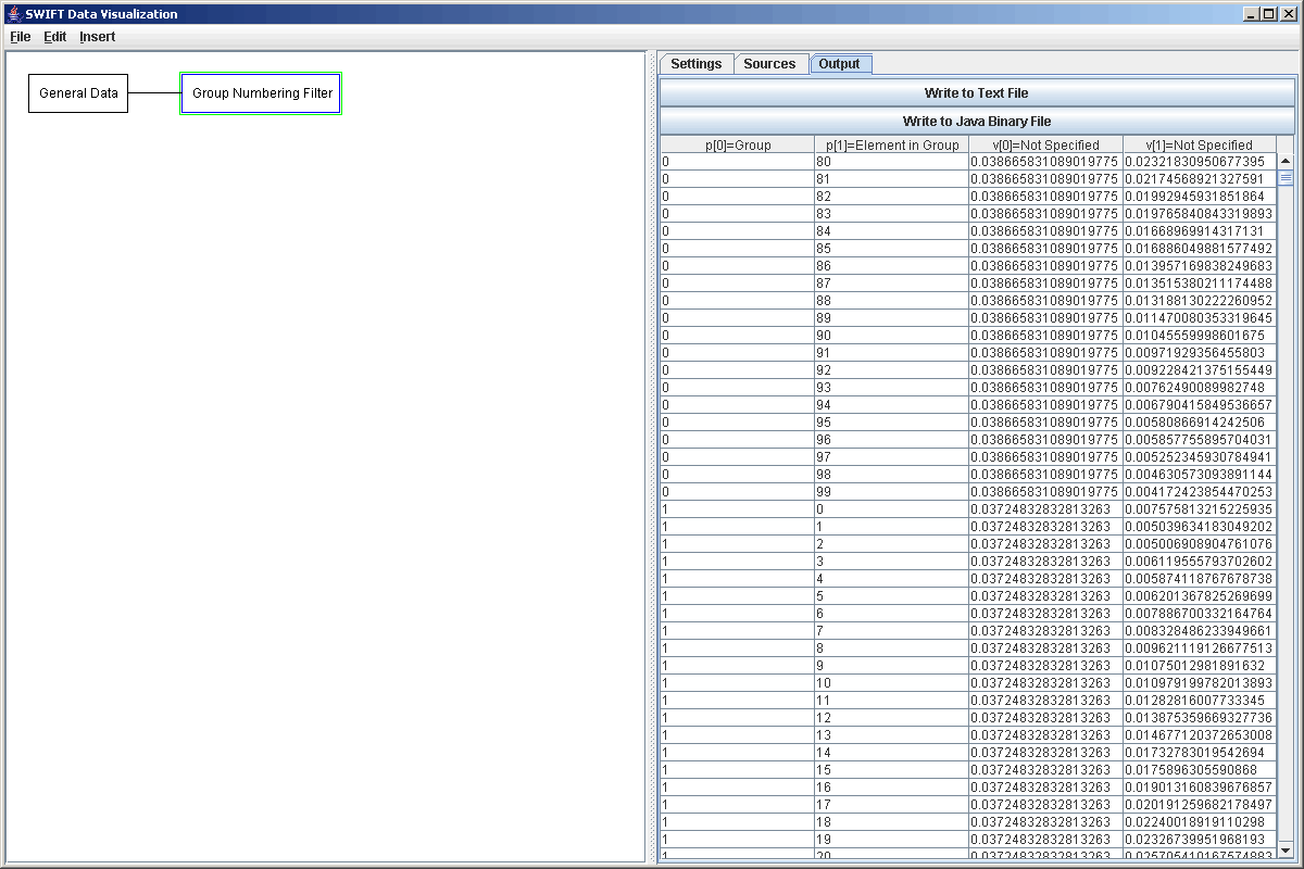
The figure above shows the output of the Group Number filter. It has been scrolled down to show the break from group 0 to group 1. Notice that the first parameter gives what group the element is in and the second parameter is what element of that group it is. It is the second parameter that we care about here.
This data file had quite a bit of data in it so to make reasonable plots and keep things running smoothly we should put in a selection filter. This could have been put before the Group Numbering filter, but we will put it after. For reasons beyond this tutorial that would be more efficient if we change the selection frequently and less efficient if we don't. For this example, we will select Y values between -1 and -3 with a selection formula of "v[0]<-1 and v[0]>-3".
For the next step in the process, we could pass this through a Function Filter to calculate proper radial distance values from the group number parameters given here. If we were going to send these values to multiple places that would actually be a smart thing to do. The Function Filter is covered in our next tutorial though and we aren't going to send this data to other locations so instead we will skip right to sending it to a plot. We add the plot to the graph, then add a Plot Area. Next we go to Data Sets and add a Rectangular Surface, then remove the Scatter Plot that was put there by default. Because of what we want to plot, we change the formulas as shown in the figure below.
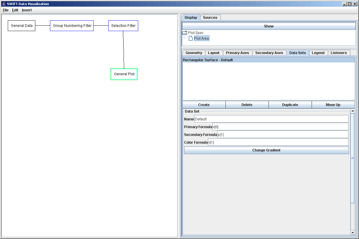
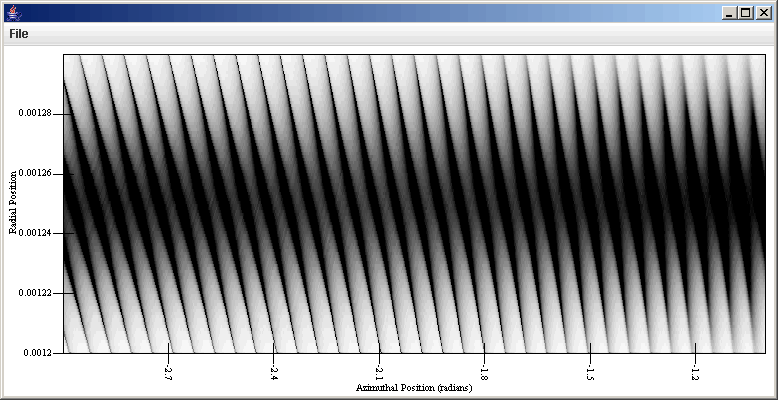
This simply uses the integer enumeration of the bins as the value of the secondary axis. To create a more meaningful plot, this can be edit to be radial_min+p[1]*radial_width/99, where radial_min is replaced by the inner edge position of the simulation and radial_width is the width of the simulation region. Doing that and putting labels on the axes produces the plot shown below which displays wakes in a perturbed ring..
Now we turn to a different data file format and how to load it in with the General Data source. We will add another General Data source to our plot and again set it to use a special format. This time, the file that we are reading is again a text file and for very similar data. However, in this case, the information was binned by grouping nearby particles and so the number of bins varies with the number of particles. In this case the output has the following format. It starts with an azimuthal position (Y), then has an integer for how many bins there were. After that the proper number of lines with each line having the average particle positions and velocities in cartesian coordinates. The format string to read this could be written as follows "v[0]=r num=i {num v[1..6]=r}". There are some new features introduced here that weren't used in the previous format string. First, the term num=i does much what it looks like, it read an integer and stores the value with the name num. We could have stored this as a parameter, but that would take up space in memory and we aren't really going to use it. We only need that number to tell us how many lines there are before the next timestep. The term v[1..6]=r is also something new. The meaning should be fairly obvious. It is a shorthand for "v[1]=r v[2]=r v[3]=r v[4]=r v[5]=r v[6]=r". Notice that num can be used as the first expression in the curly braces. This space can hold a variable, a parameter, or a value (which would be trucnated to an int). It can not currently include arithmetic expressions though that might be added in the future.
If the above string were entered as the format and we clicked read, the entire file would be read in and we would have the average positions and velocities in all 3 dimensions. In this case, the data file is almost 1GB in size and we really don't want to read in the whole thing. Also, we aren't interested in all of the values in the file. It turns out that right now we only want to plot information for the cartesian x coordinate, which happens to be radial position. In order to not read the whole file and to store only the x values we can use the following modified formula "{4000 v[0]=r num=i {num v[1]=r r r r r r}}". Here we have placed the entire string from above inside curly braces and told it to read only 4000 times so this will only get the first 4000 timesteps. In reality, the format strings we used earlier were put in curly braces with a # symbol in the first slot. This tells the General Data reader to keep reading that until it gets to the end of the file. This could be put in an interior bracket if what was read before it was something like header information. Notice also the free standing r's. These tell the program to read a real, but not store it anywhere. This way, our elements will have only two value in them and we use a lot less RAM. If we wanted the other values we could certainly edit this string and read them in. The figure below shows the new General Data element and the format string.
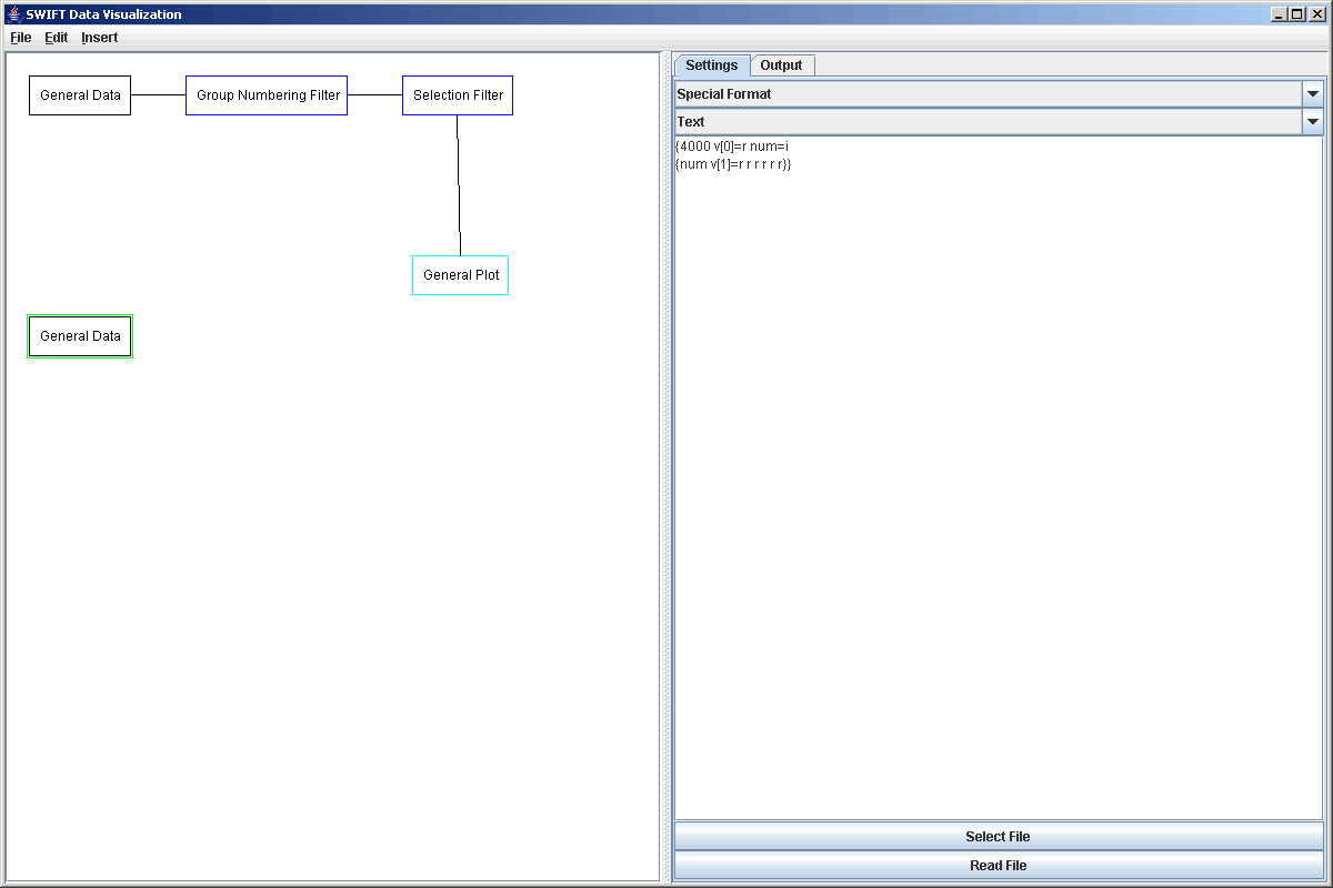
Notice that a linefeed was inserted in the interest of making the format string more readable. White spaces can be inserted between terms as the user sees fit. Even though this only read 4000 timesteps, each timestep had roughly 200 data points in it so we still come away with over 800,000 elements. That's too much to plot directly and come up with anything meaningful. So again, we will send this information through a selection filter. This time we'll take azimuthal positions between -1.5 and -2.5 radians with the formula "v[0]<-1.5 and v[0]>-2.5". Now we can take that data straight to a plot.
This time, after adding the plot and the plot area in it, we want to replace the scatter plot with an Averaged Surface plot. The averaged surface is much like the Rectangular Surface, with the exception that the panels it draws don't have to be rectangular. This plot type was written for plotting exactly this data and the properties panel for it has quite a few options that are shown in the figure below.
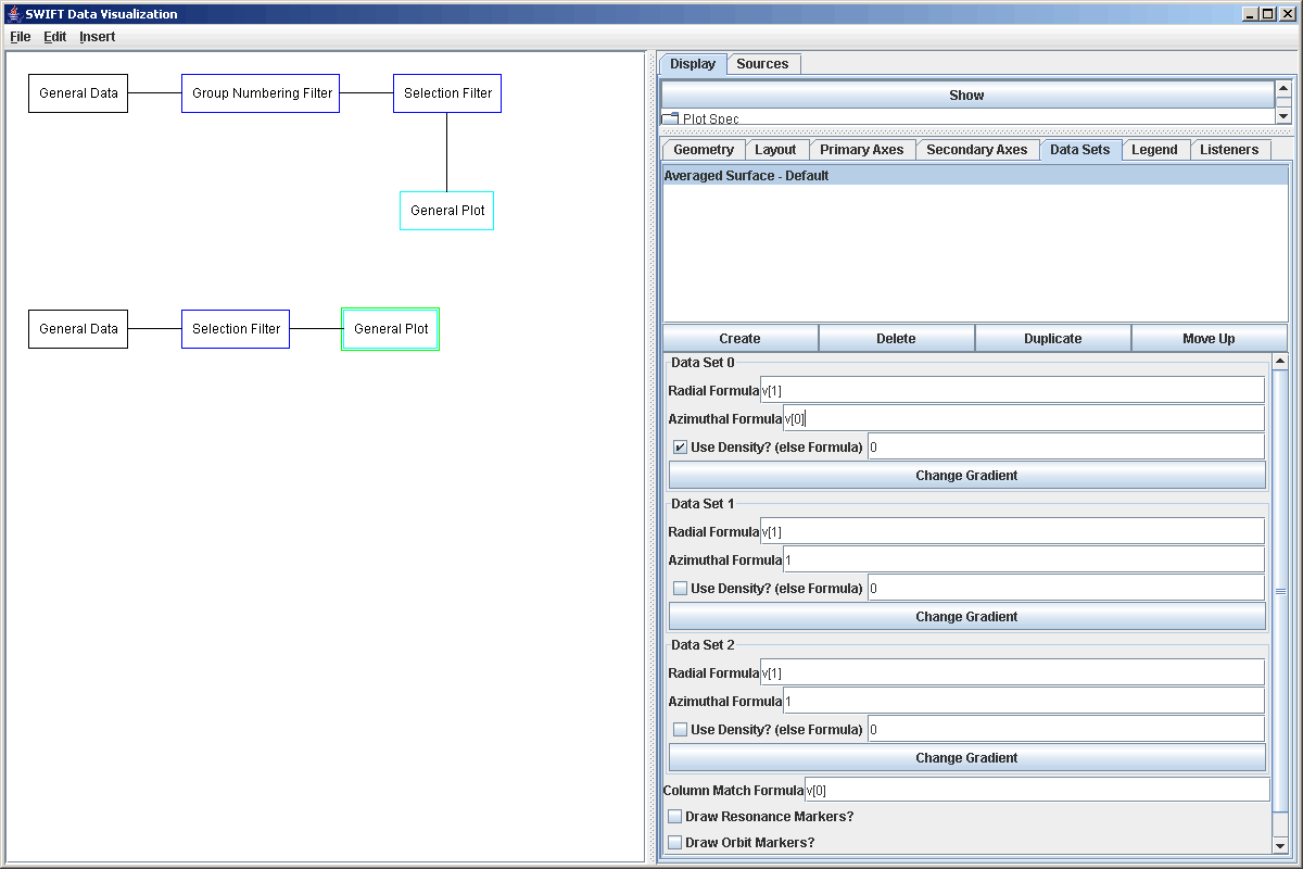
This plot style allows you to overplot 3 data sets and you can pick a gradient for each one. You specify the radial and azimuthal formulas for each. In this case, radial is v[1] and azimuthal is v[0]. You can entere a formula to use for the coloring of the gradient, or click "Use Density". When Use Density is clicked, the formula is ignored, and the regions are colored based on how distant adjacent elements are. If the formula is 0 and the Use Density box is not checked, nothing will be plotted for that set. Due to the fact that this was used with ring data, you can also select to put in markers for Lindblad resonances as well as vertical lines at locations where the azimuthal position is 2*PI*n. The figure below shows what this looks like with some labels on the axes. It is very similar to what we had in the previous plot. This one is not as blocky though and though it can't be seen well here, it has higher resolution in the higher density areas.

The last data file that we want to work with here is a binary data file for a full dump of a ring simulation. The format of this file is rather simple. It has a single integer at the beginning telling it how many bodies are in the file. That is follwed by the proper number of x, y, z, vx, vy, vz tuples, where each is written as a 64-bit double precisions number. That is followed by the same number of double precision values for the radii of the particles. This actually shows a limitation of the General Data source. It has to read in full elements at a time, so we can't read this format and get the particle radii in the same elements as the positions of the particles they belong to. To do that would require either a special data source (see the page on extending SWIFTVis for this) or we could preprocess that data to alter the order of things. For this particular example, we will do neither, we will live with not having the radii because for the simulation we will look at, all the particles were the same size.
In order to read this in, we need to add another General Data source and again we tell it to use a special format. This time we tell it that the read style is binary instead of text. Unlike the previous data files, we must leave some of this file unread because it wouldn't make sense. Also, there are again certain values that we don't care about. For this example we will care only about x, y, and vx (because you might be getting tired of just seeing density plot). The format string to do this is as follows: "{1 num=i*4 {num v[0..1]=r*8 r*8 v[2]=r*8 r*8 r*8}}". The outer curly braces with the 1 will prevent it from trying to read another int and some positions from the radii at the end of the file. The stand-alone r's skip z, vy, and vz. We also specify the exact size of the reals and the integer in bytes. By default, i would read a 2 byte integer and r would read a 4 byte floating point. This is the default because it is what SWIFT uses most. The data file being used here uses a 4 byte integer and double precision floating points.
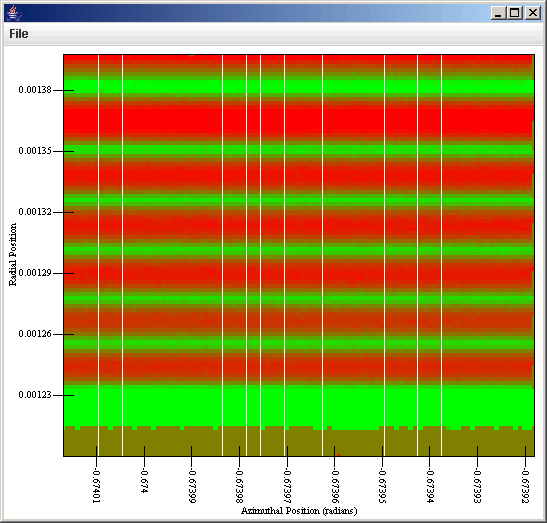
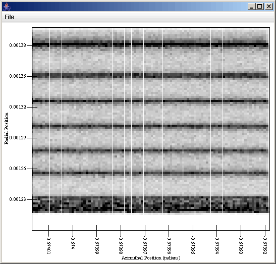
We can select the file, read it in, and check the Output tab to make sure that the values we have are roughly correct. This particular file has 1,000,000 particles in it so plotting is straight to a scatter plot would produce something that has no meaning to us. Instead, we will put it through a Binned Filter so that we can group together particles are are adjacent in the x, y-plane. We have to add a second binning coordinate for the y value and set the ranges on both x and y to be appropriate to the data. By default, the binning does a count of how many elements are in each bin, we will keep that and add a second bin value that computes the average of vx using the formula v[2]. The figure below shows the properties of the Binned Filter after we have put in the proper values.
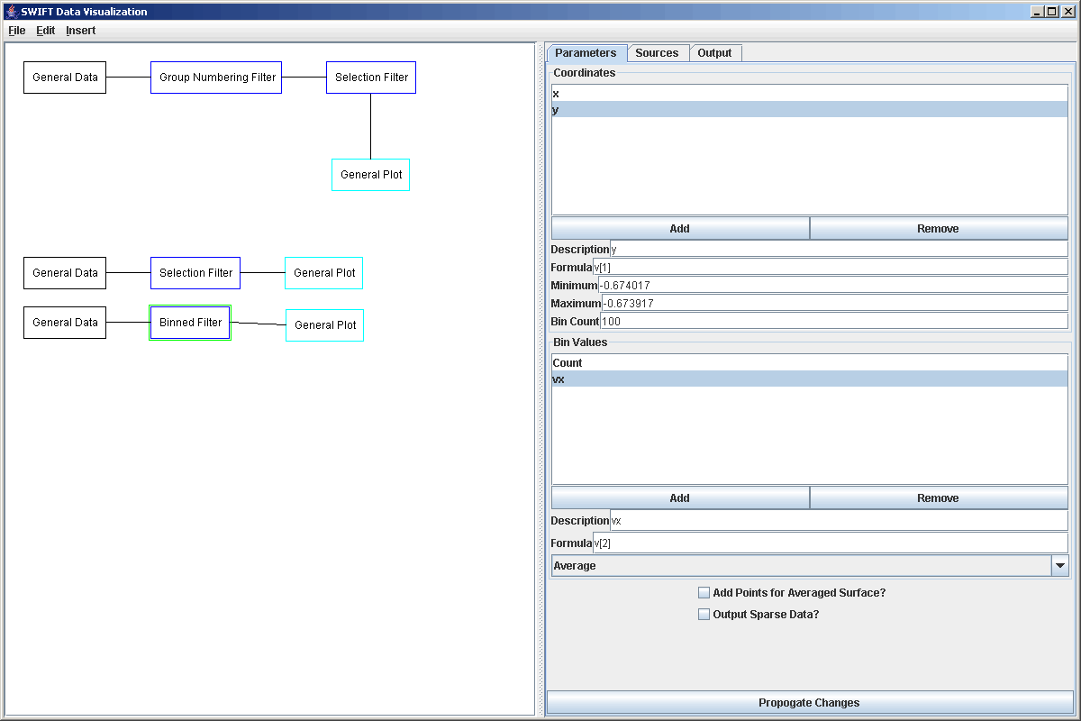
This can now be sent to a plot that has a Rectangular Surface style set up. If we plot vx with the proper gadient we get the first plot. If we plot the counts with the proper gradient we get the second plot.
At this point you should understand many of the abilities of the general data source and what you can use it for. You also have some idea of the limitations that it has. In the next tutorial, we will look at how you can use SWIFTVis to transfor data or do simply thing like plotting functions.
For more information on the aspects of SWIFTVis discussed in this tutorial, see the pages for General Data Source, Rectangular Surface Plot, Binned Filter, and Average Surface Plot.