Plotting Functions and Transforming Data
The fact that SWIFTVis can work with functions should be no surprise at this point as the use of formulas has been a constant theme in all the tutorials. In this tutorial we look at some simply uses of SWIFTVis that can help with any number of activities. The key aspects are the introduction of the Function Filter and the Sequence Source.
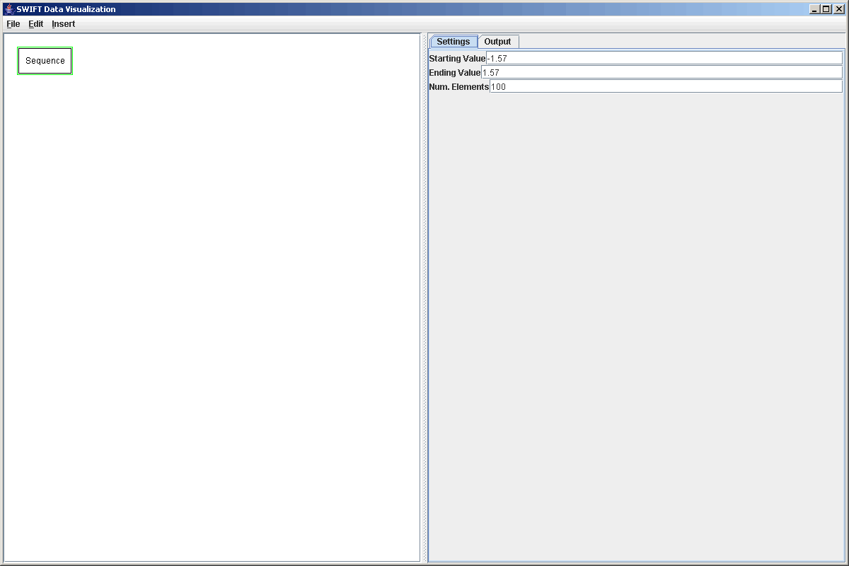
Obviously, SWIFTVis was written primarily to allow people to analyze simulation output from SWIFT and SWIFTER. However, it can be used for many other tasks and sometimes, in the process of analyzing data you want to ask other simpler questions. Also, sometimes you want to bring numbers into the SWIFTVis system that aren't part of your data file. This tutorial discusses ways of doing that. To begin with, let's look at how we can get teh values for and plot a simple function. Say we want to plot sin(x). We already know that if we have values for x in as a value in some elements, we can type in something like sin(v[0]) to get the sines of those values and that formula can be entered in many different places. What we can't do well right now is get a sequence of x values to use. We could certainly go outside of SWIFTVis and type in a text file with the numbers we want, then use a General Data source to read that file in. That's a pain though so SWIFTVis provides a Sequence Source. This is a data source that doesn't pull from any file, instead it simply provides elements with one value in them and that value will be evenly spaces numbers from some minimum to some maximum. To plot sin(x) we might want to get 100 values between -1.57 and 1.57. The figure below shows the properties of the sequence source with these values.
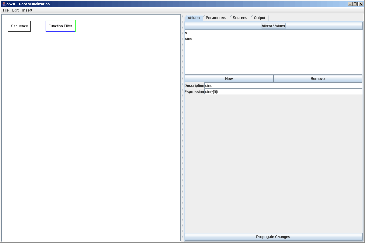
Since we can enter formula directly into the primary and secondary fields of the scatter plot, we could easily just go straight to a plot here and put v[0] as the primary value and sin(v[0]) as the secondary value and we could see our sine function. However, we will assume here that we might want to do something beyong just a simply plotting of this function so we want to have an element of our graph that has v[0] as the values of x and v[1] as the values of sin(x). To do this we use a Function Filter. The Function Filter does exactly what the name implies, it applies functions to things and in this case, uses those functions to calculate new values and parameters for elements. The Function Filter's property panel has four tabs. Two of those are the standard Sources and Output tabs. The other two are for Values and Parameters. Each of those has a button at the top that provides you with a simple way to copy the inputs from the source. Below that button is a list of the current values/parameters that you can select, add to, and remove from. When you select one, the properties for it come up below the list and you can edit the name and formula for each one. In our case, the input only has one value so we can click "Mirror Values" to quickly bring it across. We might even want to change the name "Sequence" to "x" to fit with this example.
Now we want to add a new value which we do by clicking the "New" button. This creates a value called "New Value" with the formula of 1 by default. We can change the name to sine and the formula to sin(v[0]). The figure below shows the properties panel after we have done this.
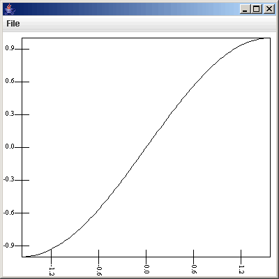
Clicking on the Output tab shows the values that are being passed along. We will instead view these by adding a plot and doing a plot of the function. We add the plot, add a plot area to it, and just selecting show gives us something very close to what we want to see. The only problem is that it is all points without lines connecting them. If we set the symbol size formula to 0.0 and select "Connect with lines", we get a plot that is closer to what we probably wanted to see as shown in the figure below.
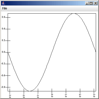
We might decide that this isn't really enough of the function so we could go back to the Sequence Source and edit the beginning and ending values to be -3.14 and 3.14. The changes automatically propogate down to the plot which changes to look like the figure below.
Of course, the Function Filter can also be used with SWIFT data as well. For example, we might want to calculate the Tisserand parameter of the test particles in our simulation. If we load in a bin.dat using the Binary Position source we could add a Function Filter and put in a new value with the formula "1/(a*v[1])+sqrt(a[1]*(1-v[0]**2))*cos(v[3])". Because we can also remove values with a function filter, we could go without the OMEGA, omega, and M values from the bin.dat file and have the Tisserand parameter by the 4th value.
For the common, yet complex transformation of changing coordinate systems, there is a different filter that you can use instead of typing in the formulas into a function filter.
Note that the function filter can consume a fair bit of memory. Because the elements are being changed, the Function Filter does not reuse the elements of the input filter. Instead, it must create new elements. The Function Filter will likely double the memory use of the primary source it pulls from. So, if the input source is very large, then that could mean taking up another sizable chunk of memory. If the functions are complex or slow though this is a space vs. speed tradeoff because the Function Filter will evaluate them once for each element and save the values while typing the formulas of a plot of some other element would reevaluate them every time the element is forced to update.
At this point you have now seen how a Sequence Source can be used with a Function Filter to add arbitrary functions into the SWIFTVis system. The function filter can also be used to do more general transformation of data in the SWIFVis system. We will revisit the use of the Function Filter in the next tutorial in order to help find particles in a system that are in resonance.