Elements and Basic Information
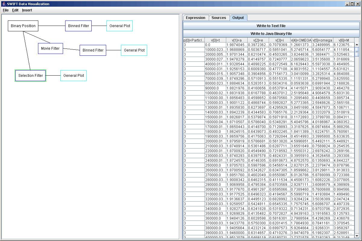
The way SWIFTVis works is that information is passed through the system in the form of elements. Each element can store a number of parameters and values. The parameters are integers while the values are single precision floating point numbers. These are referenced as zero indexed arrays. The following screen shot shows the output of an example filter in SWIFTVis.

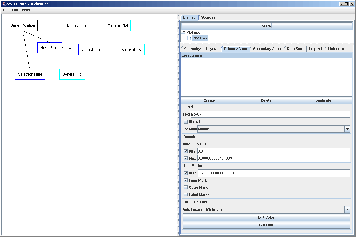
The elements are passed from a source, through zero or more filters, to a plot. The way is which the elements flow through the system is depicted to the user in a graph. Clicking on one of the boxes in the graph brings up the options for that particular graph element. For example, the figure below shows a small graph in which information from a SWIFT binary data file is passed through a binning filter to a plot. Notice that the plot box is outlined showing that it is selected. The options for that plot appear on the right side panel.

You can also select multiple graph elements at a time by either drawing a box around them, or by holding Ctrl while clicking on elements. Selected elements can be deleted, cut, or copied and elements that are cut or copied are put in a clipboard so that you can paste them.
The real work of processing the information is done in the filters. These do many different things, depending on their type. What they share in common is that they accept data from one or more sources or filters and then send data out to one or more plots or filters. The data that is sent out might be a subset of what was sent it, or it might transform the incoming elements to produce new elements to output. By combining the filters in different ways, you can explore different aspects of your data sets easily.
The plot element in SWIFTVis are also rather fully featured. While it might not replace your standard plotting package, it can produce fairly high quality output. It's true purpose though is to allow you to visualize your simulation data quickly and efficiently. You can place multiple plots in one area and each plot can display multiple data sets using the same or different axes. The way in which data is displayed in the plot area can also be changed with the use of different plot styles. For more information on the options available for plotting, see the plotting page.
A large part of the power of SWIFTVis comes from the ubiquitous ability to enter in formulas. In general, the user is almost never constrained to specifying a single parameter or value from an element. Instead, one is able to input general formulas that can include parameters or values from elements. The use of formulas was put into SWIFTVis because it is impossible for us to foresee all of the analysees that users will want to perform on their data. Instead, we have tried to provide a flexible method for users to manipulate there data inside the system dynamically without having to alter code or recompile. The foundation of this is based on two formula classes in the SWIFTVis package.
The DataFormula class is used to do numeric transformations and returns floating point values. These are also used with a BooleanFormula class that can compare values to give true or false values. Because the DataFormula is the foundation, we will discuss the format of it first.
The formulas can use standard mathematical functions in them in normal infix notation with parentheses. That is to say that operators go between operands, just like you normally write on paper. It also allows you to specify data from one of the inputs. Typically the functions will be working on a particular DataElement though it is possible to refer to earlier or later elements as well. The format for referring to data elements is d[#].p[#] for an integer parameters or d[#].v[#] for a value. The # in the d subscript is which source for that sink to use. The # in the p or v subscript is which parameter or value. To refer to values of earlier or later elements you can use a format like d[#].v[offset][#]. Here the offset is how many data elements forward or backward to look. The shorter form above is equivalent to d[#].v[0][#].
Because many situations will involve only one data source, you can also use a shorter notation where the d[#]. is dropped off. In this case the [0] source is assumed. So v[3] is equivalent to d[0].v[3]. Note that all indexes are zero referenced so v[3] is the fourth value in an element. Most elements will allow you to easily view the sources they take in so you don't have to remember what the order of the data sources is and what values mean what.
You can also refer to other elements in "groups" around a given element,
such as all elements in the same timestep as the current one. You do this by
providing a group specification and selection before the formula. The group
specification has the following format {group formula, selector 1,
selector 2,
}. The group formula has the format of a formula as described here.
Consecutive elements with the same value for this formula are put in a "group".
For example, you can group all the elements of a bin.dat file by timestep by
using the formula v[0]. The selectors are boolean formulas or have the form min ... or max ..., where ... is a standard numeric formula. If it is a boolean expression, the first element
of the group that makes the expression true is selected. Otherwise the element that evaluates to the smallest or largest value will be selected. If there is a tie, the first one will be chosen. The selected elements
are referred to with primes/single quotes. So if you have a bin.dat file read in where Jupiter
has a particle ID of -2 and Saturn has a particle ID of -3, you could use them
in a formula as follows: {v[0],p[0]=-2,p[0]=-3,max v[1]}v[5]-v'[5]-v''[5]+v'''[5]. In this formula,
v' gets values for Jupiter in the group an element resides in, v'' gets values
for Saturn, and v''' is the body with the largest semimajor axis. Because of the way that selections are cached, the selections will not reevaluate if all the elements are in a single group (or if the group formula is a constant), even when the input data is changed.
If you want to refer to "constants" that are coming from your data you can use a slightly different syntax. When SwiftVis is processing, it sees an entry of the form d[#].p[#][#] or d[#].v[#][#] and that entry will be run through all the valid indexes for the input as determined by the element in question. If you replace the d with a c, it will always refer to the first element from that data source. This syntax does not support selection for special indexes in groups. In cases where that isn't required, this can be a shortcut so that the user doesn't have to use a constant filter. As with the d expressions, the offset is optional. It can be used to take values or parameters from other elements in the data set, but the user must know the index they want.
These formulas support the operators +, -, *, /, %, and ** as well as the ternary
operator ?: for doing conditionals (See BooleanFormula below for the format of the
conditionals). Note that % is defined as modulo in the C-family languages, the
?: operator is a shorthand for conditional logic in an expression, and ** is
exponentiation as in Fortran. The ternary operator has the highest precidence (excluding operators between the ? and : which are effectively in parentheses).
Other operators follow normal mathematical precendence with % at the same level
as * and /. You are also allowed to use some standard functions in your expressions.
The table below lists all of the functions you can call in a formula along with their arguments and a description. So if you had data with angles and distance from the origin you could transform
it to Cartesian coordinates with expressions such as v[0]*cos(v[1]) and v[0]*sin(v[1]). The index function doesn't take any arguments and can be used with or without following parentheses. It gives you the index of the current element in the source. This is useful for making cummulative distributions. There is also an scm function that allows you to embed SVScheme code inside of a general formula and PI can be used for that constant.
| Function/Const | Description |
|---|---|
| abs(x) | Absolute value. |
| acos(x) | Trig arccosine. |
| asin(x) | Trig arcsine. |
| atan2(y,x) | Trig arctangent with two arguments. |
| cbrt(x) | Cubed root. |
| cos(x) | Trig cosine function. |
| cosh(x) | Hypercosine of x. |
| exp(x) | e^x |
| floor(x) | Floor of x. |
| hypot(x,y) | Returns sqrt(x^2+y^2) without intermediate overflow or underflow. |
| index | The index of the current element. The first element from a source has index 0. |
| log(x) | Natural log. |
| log10(x) | Log base 10. |
| log2(x) | Log base 2. |
| max(x,y) | Maximum of x and y. |
| min(x,y) | Minimum of x and y. |
| numElements[(s)] | The total number of elements coming from a source. The argument specifies which source. If no argument is given source 0 is assumed. |
| numParams[(s)] | The number of parameters in the current element from a source. The argument specifies which source. If no argument is given source 0 is assumed. |
| numValues[(s)] | The number of values in the current element from a source. The argument specifies which source. If no argument is given source 0 is assumed. |
| PI | The constant pi. |
| rand(x) | Random number between 0 and x. |
| round(x) | x rounded to nearest integer. |
| scm(code) | Runs the specified code using the SVScheme interpreter. |
| sin(x) | Trig sine function. |
| sinh(x) | Hypersine of x. |
| sqrt(x) | Square root. |
| tan(x) | Trig tangent function. |
To help keep the speed of the application at good levels while allowing this flexibility, the DataFormula class parses the formula out to an expression tree and all evaluations are done on the tree itself. The evaluation process does not involve any string operations.
The format listed above works well for calculations and converting things.
Many of the filters also require the ability to do logical operations on these
values. For this, we have added the BooleanFormula class. This class is intended
to allow users to type in formulas that use parameters or values from elements
that evaluate to Boolean values. The operators that are understood by this class
are the following logical operators: =, <, >, <=, >=, &, and, |, or, ^, xor,
!, not. Note that for the Boolean operators you can use C-ish characters or
full names. Also note that the characters are single, unlike in C, but they
are still short circuit. Also note that equality is a single '='. All formulas
can use parentheses to specify order of operation. Without them the comparisons
have highest precedence, followed by and, or, and xor in that order. At the
same level they all go left to right as one would expect.
The comparisons compare two numerical expressions. Those expressions should
conform to that used by the DataFormula class. So if someone wanted an expression
that was true for all planets read from a SWIFT binary file, but not for test
particles, they might write p[0]<0. To see if a certain point was more than
a given distance from the origin the expression might look like sqrt(v[0]*v[0]+v[1]*v[1])>2.
As with the DataFormula, "group" selection information can be provided at the beginning of a BooleanFormula. This way you can provide a selection for all elements of bodies within 1 AU of Jupiter that might look something like the following.
{v[0],p[0]=-2}abs(v[1]-v'[1])<1
Alternately, instead of using abs one could use boolean operators as such:
{v[0],p[0]=-2} v[1]-v'[1]<1 & v[1]-v'[1]>-1
It is also possible to put SVScheme code into any formula in SWIFTVis. You do this with the scm function. It should be followed by a valid SVScheme expression in parentheses. So, for example, 6*scm(+ 2 3) would return the value 30. This is a very inefficient way to get 30 though and the use of scm in formulas should be avoied unless it truly provides you with extra power. The scm function is also usable in boolean formulas and in that case it should return a boolean valued expression. Writing long SVScheme functions into the small text fields where most formulas are edited would be a bit of a pain. For this reason, you will most likely write longer functions in the Options dialog and call them in your formulas. For information on this, see the SVScheme Tutorial.
To see how the data and boolean formulas are used in SWIFTVis, read the other tutorials and the descriptions of the various filters.
We look at some uses for these formulas in the plotting and analysis of the data in a bin.dat file in the next tutorial.